Simulation models
For a more detailed representation of temperature effects and pressure losses in the district heating network, linear optimization models do not suffice. In this situation, a simulation model can be the right choice.
Scope
The following questions can be addressed using a simulation model:
How do the heat losses in the network depend on the temperatures of inlet and return pipes and ambient temperature?
How much energy is necessary for the pumps to overcome the pressure losses in the network?
How do these properties behave if the supply temperatures change?
To answer these questions, data has to be present or assumptions have to be made about the pipe’s physical properties and the temperature drop at the consumers. Have a look at the overview table to learn about all the variables and parameters involved.
Conversely, if these are not known, running an optimization model would be the better choice. It is also possible to couple the two approaches, running an optimization first and then investigating the detailed physical behaviour. To learn about this option, please refer to the section model coupling.
Currently, the available simulation model does not handle transient states (i.e. propagation of temperature fronts through the pipes). The model evaluates a steady state of the hydraulic and thermal physical equations. This also means that consecutive time steps are modelled independently and the behaviour of thermal storages cannot be represented. A dynamic simulation model may be implemented at a later point in time.
Usage
To use DHNx for a simulation, you need to provide input data in a defined form. The basic
requirements are the same for all ThermalNetwork s, but some input data is specific to the
simulation:
tree
├── consumers.csv
├── pipes.csv
├── forks.csv
├── producers.csv
└── sequences
    ├── consumers-mass_flow.csv
    ├── consumers-delta_temp_drop.csv
    ├── environment-temp_env.csv
    └── producers-temp_inlet.csv
To run a simulation, create a ThermalNetwork from the input data and simulate:
import dhnx

thermal_network = dhnx.network.ThermalNetwork('path-to-input-data')

thermal_network.simulate()
Figure 1 shows a sketch of a simple district heating network that illustrates how the variables that are determined in a simulation model run are attributed to different parts of a network. Pipes have the attributes mass flows, heat losses and pressure losses (distributed and localized). Temperatures of inlet and return flow are attributed to the different nodes. Pump power belongs to the producers which are assumed to include the pumps. Variables that describe the network as a whole are global heat losses and global pressure losses.

Fig. 1: Schematic of a simple district heating network and the relevant variables for simulation.
The above-mentioned variables can be found in the results of a simulation, which come in the following structure:
results
├── global-heat_losses.csv
├── global-pressure_losses.csv
├── nodes-temp_inlet.csv
├── nodes-temp_return.csv
├── pipes-dist_pressure_losses.csv
├── pipes-heat_losses.csv
├── pipes_loc_pressure_losses.csv
├── pipes-mass_flow.csv
└── producers-pump_power.csv
Underlying Concept
Name |
Math. symbol |
Unit |
Common values |
|---|---|---|---|
Variables |
|||
mass flow |
|
|
|
mean flow velocity |
|
|
|
pressure |
|
|
Nominal pressures PN16 or PN25 |
pressure difference |
|
|
max. |
pump power |
|
|
|
temperature |
|
|
Inlet pipe: |
ambient temperature |
|
|
|
heat flow |
|
|
|
Water properties |
|||
density |
|
|
|
spec. heat capacity |
|
|
|
dynamic viscosity |
|
|
|
darcy friction factor |
|
– |
|
Reynolds number |
|
– |
|
Parameters |
|||
pipe’s length |
|
|
|
pipe’s inner diameter |
|
|
Nominal diameters DN25 - DN250 |
localized pressure loss coefficient |
|
– |
|
standard acceleration due to gravity |
|
|
|
altitude difference |
|
|
|
pipe’s absolute surface roughness |
|
|
|
heat transfer coefficient |
|
|
|
spec. heat loss per meter |
|
|
|
pump efficiency |
|
– |
|
electric pump efficiency |
|
– |
|
hydraulic pump efficiency |
|
– |


 |
| 


 , Return pipe:


 at
at 


 at
at 
 at
at 


 ,
, 


 )
)
 (sometimes just


The following equations are related to a single pipe.
Hydraulic equations
A pressure difference between two ends of a pipe occurs because of three effects:
distributed pressure losses along the pipe’s inner surface
local pressure losses at distinct items,
hydrostatic pressure differences because of a difference in height.
All three effects can be captured in this formula:

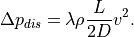
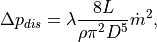
Distributed pressure losses
The Darcy-Weissbach-equation describes distributed pressure losses
 inside the pipe:
Together with the flow velocity

it can be written to:
where the darcy friction factor 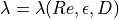 depends on the Reynolds
number
depends on the Reynolds
number  , the pipe’s surface roughness
  and the pipe’s inner diameter
 . The Reynolds number is a dimensionless quantity characterizing fluid flows and is defined
as follows:
. The Reynolds number is a dimensionless quantity characterizing fluid flows and is defined
as follows:

 is the dynamic viscosity of water.
In a pipe, flow is laminar if  < 2300 and turbulent if > 4000.
In district heating pipes, flow is usually turbulent. The turbulent flow regime can be further
distinguished into smooth, intermediate and rough regime depending on the pipe’s surface roughness.
< 2300 and turbulent if > 4000.
In district heating pipes, flow is usually turbulent. The turbulent flow regime can be further
distinguished into smooth, intermediate and rough regime depending on the pipe’s surface roughness.
[1] provides the following approximation formula for  :
:

A more accurate approximation of the Colebrook-White-equation for flow in pipes is given by this formula:
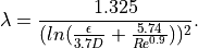
Local pressure losses
Local pressure losses are losses at junction elements, angles, valves etc. They are described by
the localized pressure loss coefficient  :
:
It is assumed that each fork has a tee installed. According to [2], localized pressure losses occur
downstream of the element that causes these losses. The values of the localized pressure loss
coefficient were taken from [3]. In case of a tee which splits the stream,
is 2. In case the streams join, is 0.75.
It is also assumed that each consumer has a valve installed. Due to the complexity of determining the localized pressure loss coefficients, these losses have not been considered so far.
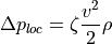
Hydrostatic pressure difference
The hydrostatic pressure difference is calculated as follows:
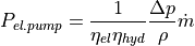
Pump power
The mass flow in the pipes is driven by the pressure difference that is generated by pumps.
The pumps have to balance the pressure losses inside the pipes. The pump power thus depends on the
pressure difference along the inlet and return along one strand of the network,  ,
the mass flow
,
the mass flow  and the pump’s efficiency
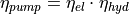 .
.
In a network consisting of several strands, the strand with the largest pressure losses in inlet and return defines the pressure difference that the pumps have to generate. The underlying assumption is that the consumers at the end of all other strands adjust their valve to generate the same pressure losses such that the mass flows that are assumed are met.
Thermal equations
The temperature spread between inlet and return flow defines the amount of heat that is transported with a given mass flow:

A larger temperature spread allows smaller pipe’s diameters, which reduces the investment cost of new pipes or increases the thermal power of existing pipes.
Heat losses
Heat losses depend on temperature level, mass flow and pipe insulation. Especially the representation of the heat losses depends a lot on the level of detail of a model. As mentioned above, in the current implementation, the thermal state of the network is assumed to be in steady state conditions. The temperature at the outlet is calculated as follows:
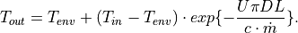
Where  and
and  are the temperatures at the start and end of the pipe,
 the environmental temperature and
  the thermal transmittance.
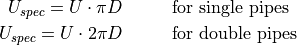
In data documentation of pipes in a district heating, you often find the value of the specific heat
loss per meter ![U_{spec} [W/(K m)]](_images/math/7de60d2b920ccce1d170a737bcef324ba93b3faf.png) .
.
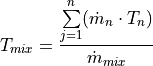
The temperature of the return flow at the fork is calculated assuming ideally mixed flows, where no
heat losses occur and the heat capacity is constant. The temperature of the mixed flow
 is calculated for a number
  of inlet flows, that are ideally mixed, using
the following equation:
of inlet flows, that are ideally mixed, using
the following equation: